
Centrifugal Pump Design Tool
Preliminary hydraulic impeller design and DXF export for further CAD work.
Opens the Streamlit application in a new tab. After a long period of inactivity, a short reactivation may be needed.
Introduction and development status
This web-based centrifugal pump design tool is primarily intended for mechanical engineers working on centrifugal pump sizing, development and optimisation. It also enables students, lecturers and turbomachinery specialists to explore the early design process for a radial pump impeller.
The current version is in an early beta phase. It has been made publicly available to gather practical user feedback, identify possible errors and improve the calculation methodology and user guidance. Feedback from industry and academia is particularly welcome.
Unlike simple online calculators, this tool does more than calculate individual parameters. From the input data it generates a complete preliminary impeller design, including hydraulic parameters, inlet angles at hub and shroud, a meridional section, blade projection, DXF files for CAD, CSV tables and a technical calculation report.
The current version focuses on impeller design. Volute calculation is not yet included, but may be added in later development stages. The initial focus is on traceable preliminary hydraulic and geometric sizing of the impeller.
The calculation methodology follows Gülich's centrifugal pump design framework. Alongside direct calculations, the code uses iterative steps where design quantities are interdependent. One example is the coupling of inlet diameter d1, inlet flow angle β1, hub ratio k_n and suction specific speed nSS. Starting from an initial value, dependent parameters are calculated, the original parameter is updated and the process repeats until sufficient convergence is achieved.
In addition to hydraulic results, the tool outputs usable geometric data, including polar coordinates of the blade projection, meridional section geometry and exportable DXF files for further CAD work. The calculation can therefore support design, plausibility checks, teaching and further CFD studies.
The application is not currently approved for all pump types and design ranges. It applies only within defined geometric and hydraulic conditions. Outside this scope, results require critical review and do not constitute a substantiated industrial design. The next section defines the valid scope in detail.
Valid scope of application
The current tool is intended for preliminary hydraulic and geometric sizing of radial centrifugal pump impellers. Its scope is deliberately limited so that results can be interpreted clearly and meaningfully.
The tool currently covers single-stage, single-suction radial pumps with closed impellers, axial inlet and backward-curved blades. It assumes swirl-free inlet flow; pre-rotation at the impeller inlet is not included. The calculation primarily addresses water or water-like, incompressible, single-phase liquids.
The current version calculates only the impeller. Complete pump design, including volute, diffuser, bearings, detailed shaft design, strength verification, sealing concept and manufacturability assessment, is outside its scope. Nor does the tool replace full validation of NPSH, cavitation, CFD or efficiency. Simplified shaft and hub values are supplementary estimates, not a complete mechanical design.
It is not intended for multistage pumps, double-suction impellers, mixed-flow or axial pumps, open or semi-open impellers, pumps with inducers, highly viscous media, multiphase flows, gas content, suspensions, solids-laden liquids or operating ranges far from the design point.
Results are preliminary engineering estimates and starting points for further design, CAD and CFD work. Within the stated scope, the tool helps explain the key hydraulic and geometric relationships of radial pump impeller design. Outside this scope, results require critical review and are not approved as a substantiated industrial design.
Using the tool: from duty point to CAD export
- Enter duty point Q, H and n, efficiencies, blade count and thicknesses. Then check the advanced inputs; the example values are not universal design recommendations.
- Move between fields with Tab or the mouse. Enter can trigger a calculation before all inputs have been checked. Select “Hydraulik & Geometrie berechnen” only after reviewing the complete input set.
- For a deliberate β₂B specification, select “Fester Benutzerwert” (fixed user value). “Automatisch” is experimental. b₂* remains a selected design parameter; 20° and 0.055 apply only to the documented example.
- Review results together with the messages. Inspect the meridional section, inlet angles and both blade paths, then download the report, CSV tables and DXF files. Check units, viewing direction and angular reference when importing the curves into CAD.
Calculation and export
The tool calculates the main hydraulic and geometric parameters for preliminary radial impeller sizing. From flow rate, head, speed and selected design parameters, it determines inlet and outlet diameters, impeller widths, blade angles, hub and shroud inlet angles, blockage corrections and key meridional section parameters.
Alongside numerical design data, the tool generates geometry for further CAD work: a meridional section with hub and shroud contours and a top-view blade projection. The generated geometry can be exported as DXF files and used in CAD systems such as SolidWorks.
The application also provides CSV tables and technical calculation reports. Exports include polar coordinates of the top-view blade projection, meridional section points, segment information, intermediate hydraulic results and relevant design parameters. This supports preliminary impeller sizing, plausibility checks, CAD preparation, technical documentation and further CFD studies.
Who is the tool for?
The tool is intended for mechanical engineers working on centrifugal pump and impeller sizing, design, optimisation or analysis. It can be used in industry and technical education to clarify the relationships between duty point, hydraulic design and impeller geometry.
It is particularly relevant to pump developers, designers, CAD users, CFD engineers, and students and lecturers in turbomachinery, fluid mechanics and mechanical design. It helps review design decisions, prepare geometric starting data for CAD models and clearly document preliminary hydraulic results.
Universities and technical courses can also benefit. The tool enables key centrifugal pump design steps to be studied through calculated geometries, meridional sections, blade projections and DXF exports, rather than through theory alone.
Choose input parameters carefully
Meaningful use starts with a realistic duty point: flow Q, head H and speed n. These define the hydraulic task and directly influence specific speed n_q, impeller diameter, velocity triangles, suction behaviour and the resulting impeller geometry.
Select η_tot and η_h as realistic preliminary efficiency estimates. Accurate hydraulic design generally requires a loss analysis or balance, systematically estimating friction, turning, mixing, inlet, outlet and secondary losses to establish η_h more soundly. Overall efficiency η_tot also includes volumetric leakage losses and mechanical losses, such as bearings, seals and disc friction. In preliminary sizing, η_h and η_tot are often initially estimated empirically, considering pump type, duty point, flow, size, power range, specific speed n_q and expected manufacturing quality.
Blade count z affects blockage, blade loading and flow guidance. Select it together with outlet width b2, outlet angle β2B, blade length and duty point. A generic blade count is not a universal design requirement; use suitable empirical data and relevant technical literature for the specific case.
Inlet edge thickness e1 and outlet edge or blade thickness e2 must suit a realistic impeller design. Greater thickness reduces free flow area; smaller thickness must be checked against strength and manufacturing methods. Agree manufacturing-specific minimum thicknesses with the manufacturer; no universal minimum can be specified here.
Incidence angle i1 is entered manually and affects inlet metal angle β1B at hub and shroud. Justify it from the inlet flow, design methodology and operating range. A single guideline value does not replace checking inlet geometry or later validation.
The dimensionless outlet width ratio is b2* = b2/d2. Select it together with specific speed, blade count, outlet angle and blade loading. Use empirical charts within their documented scope. Width influences velocities and flow; preliminary sizing does not verify the complete Q–H curve.
Note the current tool's terminology: ‘b2* initial value’ is effectively a user-selected design value, not an automatically optimised parameter. Choose it deliberately, then assess b2, c2m, c2u, H_cal and the entire outlet geometry together.
For a deliberate β₂B specification, select “Fester Benutzerwert” (fixed user value). “Automatisch” is experimental. b₂* remains a selected design parameter; 20° and 0.055 apply only to the documented example.
Pay particular attention to H_cal when assessing results. This calculated head indicates whether the chosen combination of d2, b2, z, β2B, slip factor γ and hydraulic efficiency η_h plausibly reaches the required H. A substantial difference between H_cal and H does not automatically indicate a tool error; it often means the selected design values, especially β2B and b2*, need review.
Some other values are genuine starting values for iterative calculations, such as ψ and k_n initial values. They initialise steps that iteratively approximate coupled quantities including inlet diameter, hub ratio, inlet angle and impeller diameter. In contrast, b2* and β2B in this version are deliberate user-selected design quantities.
Never assess outputs in isolation. Check inlet geometry, inlet angles, blockage, outlet geometry, H_cal, meridional section, blade projection and DXF geometry together. Only when these appear mutually plausible should the geometry serve as a starting point for CAD modelling, CFD studies or further detailed design.
Terms and design quantities
This section explains the tool's main inputs, outputs and internal design parameters. Names follow standard centrifugal pump design terminology and notation used in technical literature.
Tool inputs
Q is pump flow rate. Together with head H and speed n, it defines the duty point for preliminary hydraulic sizing. Density ρ and gravitational acceleration g are used for power, torque and energy quantities.
H is the specified head at the design point, against which the calculated head H_cal is checked.
n is impeller speed in revolutions per minute. It influences peripheral velocities, specific speed, impeller diameter and velocity triangles.
η_tot is the assumed overall pump efficiency, used mainly for power and shaft sizing. η_h is hydraulic efficiency, used to calculate impeller head.
nSS, the suction specific speed, is a design parameter for impeller suction capability. It influences inlet sizing and is related to inlet diameter, hub ratio and inlet flow angle.
z is the number of impeller blades. It affects inlet and outlet blockage corrections and blade geometry.
i1 is the manually specified incidence angle at the impeller inlet. It is added to the calculated inlet flow direction to determine the blade inlet metal angle.
e1 and e2 are the blade or edge thicknesses at inlet and outlet, used in the blockage calculation.
b2* is the dimensionless impeller outlet width ratio, defined as b2* = b2/d2, used to determine outlet width b2.
β2B is the blade metal angle at the impeller outlet. Together with d2, b2 and velocity quantities, it strongly determines the calculated impeller head.
Key outputs
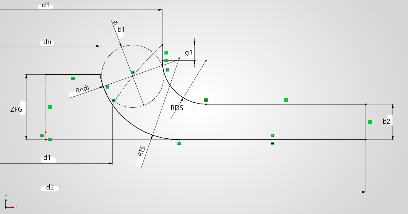
dn is the hub diameter at the inlet, or the inner reference diameter derived from shaft and hub constraints.
d1 is the outer impeller inlet diameter, measured at the shroud in the inlet region.
d1i is the inner inlet diameter at the hub, resulting from the meridional section geometry.
d2 is the impeller outlet diameter. Through peripheral velocity u2, it directly influences achievable head and is a central design parameter.
b1 is the geometric impeller inlet width. b2 is outlet width, obtained from ratio b2* and outlet diameter d2.
β1 is the inlet flow angle; β1B is the blade inlet metal angle. They are calculated separately at hub and shroud because local peripheral velocity, diameter and blockage differ.
τ1 is the inlet blockage correction factor, calculated locally at hub and shroud to account for reduced free flow area due to blade thickness e1. τ2 is the corresponding outlet factor.
The meridional section describes impeller geometry in a plane through the rotation axis. It includes hub and shroud contours and parameters such as RDS, RTS, Rndi, g1, ZFG and ZL.
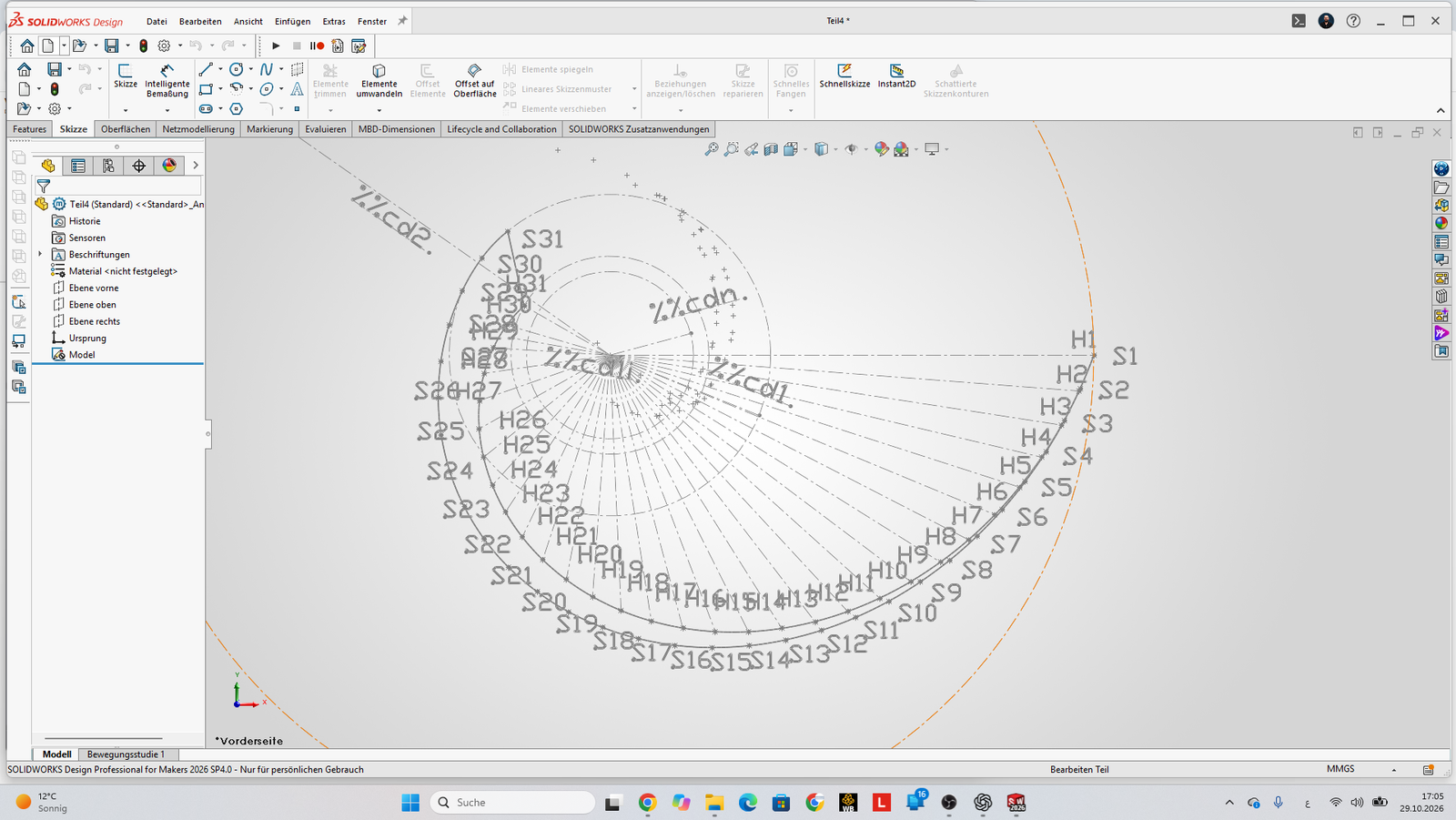
The top-view blade projection describes the projected blade geometry in polar coordinates and provides the basis for further CAD design of the blade contour.
Key values in the hydraulic report
H_cal is the calculated head of the current impeller design, determined from the outlet velocity triangle, peripheral velocity u2, circumferential component c2u and hydraulic efficiency. With the assumed swirl-free inlet, the model uses:
H_cal = ηh · u2 · c2u / g
This value shows whether the chosen combination of outlet diameter d2, angle β2B and width b2 reaches the required head H. Good agreement between H_cal and H is a key plausibility criterion in preliminary hydraulic design.
u2 is peripheral velocity at the impeller outlet. It follows from d2 and n and is a key quantity in impeller energy transfer.
c2m is the meridional outlet velocity component. c2u is the circumferential component of absolute outlet velocity and, with u2, determines the specific energy transferred according to Euler's equation.
ψ is the head coefficient. It relates head to peripheral velocity and provides a plausibility check for the selected impeller diameter.
Q_La is the design flow used for impeller sizing. It may be corrected relative to nominal flow Q by a factor intended to make the impeller design more robust.
k_n is the hub ratio or the influence of hub diameter on inlet area. In inlet sizing, it is iteratively coupled with inlet diameter and angles.
Intermediate values in the hydraulic report support both documentation and engineering checks. They help assess consistency between inlet, outlet, meridional section and blade projection.
Worked example: water, 3 m³/h, 12 m, 3000 rpm
The documented W3123000_Excel_Vergleich case connects the saved hand calculation (Calculations, row 5, and ShaftDiameter) with application screenshots dated 29 October 2026. The duty point is treated as the intended best-efficiency point; the actual best-efficiency point is not established by this assumption.
| Input / assumption | Value |
|---|---|
| Useful flow Q | 3 m³/h |
| Head H / speed n | 12 m / 3000 min⁻¹ |
| Density ρ | 998 kg/m³ |
| Overall efficiency η_tot / hydraulic efficiency η_h | 0.30 / 0.62 |
| Blade count z / incidence i₁ | 5 / 3° |
| Inlet thickness e₁ / outlet thickness e₂ | 1 mm / 2 mm |
| Power factor S_P / moment ratio M/T | 1.15 / 0.50 |
| K_m / K_t / reference stress / F0s | 2 / 1.5 / 40 MPa / 2 |
| Hub wall thickness | 4 mm |
| Suction specific speed nss / Q_La factor | 180 / 1.06 |
| k_n starting value / ψ starting value | 0.72936844 / 1 |
| Width ratio b₂* / outlet metal angle β₂B | 0.055 / 20° |
| Projection segments per path / angular reference ε₀ | 30 / 0° |
| Shroud / hub outlet inclination | 0° / 0° |
Formulae and tables use decimal points for reproducibility. Factors such as 1.06, 1.15 and M/T = 0.5 are choices for this example. The 40 MPa reference stress is not an established material property of a particular steel alloy.
On narrow screens, swipe the comparison table horizontally to see all columns.
| Quantity | Excel reference | Application: screenshots |
|---|---|---|
| n_q | 13.432124 | 13.4321 |
| P_hyd [kW] | 0.09796368 | 0.0979 |
| P_design [kW] | 0.37552744 | 0.3753 |
| d_n [mm] | 18 | 18.000 |
| d₁ [mm] | 34.634648 | 34.612 |
| d₂ [mm] | 104.188 | 104.188 |
| b₂ [mm] | 5.73034 | 5.730 |
| β₂B [°] | 20 | 20.000 |
| γ | 0.79423114 | 0.79423 |
| RDS [mm] | 5.814 | 5.814 |
| RTS [mm] | 14.286 | 14.286 |
| d₁i [mm] | 21.322 | 21.322 |
| g₁ [mm] | 2.076 | 2.076 |
| β₁B hub [°] | 27.987782 | 27.987 |
| β₁B shroud [°] | 18.215 | 18.215 |
| Hub wrap [°] | 209.898422 | 209.896 |
| Shroud wrap [°] | 230.480158 | 230.502 |
The application column reproduces the display precision of existing screenshots, not a new program run. Excel uses g = 9.816 m/s² and the application model 9.81 m/s². Iteration, blockage assumptions and geometry evaluation also differ. Close values are not independent validation of pump performance.
Hydraulic calculation method based on Gülich
The following steps explain the relationships, units and decisions in the documented example. Assumptions and applicability must be reassessed for each new case. The complete derivation and 22 source notes are available in the PDF calculation appendix.
1. Flow rate, power and suction behaviour
For f_q = 1, use useful flow in m³/s, head per stage H in metres and speed n in rpm. The internal impeller flow Q_La includes an assumed 6% leakage allowance in this example. In this convention, n_q is not a unit-independent dimensionless number.
NPSH₃ ≈ 0.377 m follows from the selected suction specific speed nss = 180. The 3% head-drop criterion does not prove cavitation-free operation. NPSHA for a real installation is not supplied. η_h = 0.62 and η_tot = 0.30 were chosen independently; the approximation η_h ≈ (1 + η_tot)/2 would give about 0.65 and does not replace a loss balance.
2. Initial shaft and hub estimate
Torque follows from design power and speed. The supplementary Excel model combines assumed bending and torsion with M/T = 0.5, K_m = 2 and K_t = 1.5. The reference stress is divided by F0s = 2. This is an initial mechanical estimate, not a fatigue or strength verification.
The model gives d_shaft ≈ 8.187 mm. After a bore factor of 1.1, a 10 mm bore is selected. With two 4 mm hub walls, d_n = 18 mm. Material, bearing spacing, load spectrum, deflection, critical speeds and connection details require separate design.
3. Iterate inlet diameter and inlet angles
The free inlet area ratio k_n depends on d_n and d₁. A starting estimate gives the normalised suction specific speed and approach angle β₁a, followed by d₁ and an updated k_n. Iterate to joint convergence. The factor 2900 applies to d₁ in mm, Q_La in m³/s and n in rpm.
The saved reference uses k_n = 0.72936844. Recalculation from d₁ = 34.634648 mm and d_n = 18 mm gives 0.72990071. The saved case is therefore not presented as a fully closed iteration. A new design needs consistent factors, angle determination and convergence criteria.
At hub and shroud, evaluate peripheral speed, free flow area and blockage locally. Since τ₁ depends on metal angle, angle and blockage are coupled. Saved factors 1.18915 and 1.17248 are reference values, not constants for other impellers. The hand calculation uses local incidence of about 3.04°; the application takes one shared value of 3°.
4. Coordinate outlet geometry, blockage and slip
b₂* = b₂/d₂ is a selected width ratio. The empirical centre line gives about 0.05077 for this case; 0.055 was selected. With d₂ = 104.188 mm, b₂ ≈ 5.730 mm. Coordinate width, β₂B, blade count z and diameter instead of optimising the angle in isolation.
λLa is the inclination between blade and disc, not β₂B. The hand model derives about 57.60° from an assumed 4° circumferential offset; agreement with the generated blade surface is not established. The documented application model uses sin λLa = 1. Identical main dimensions can therefore yield different blockage and head.
For z ≥ 3, the slip relation uses factor f₁ and diameter-ratio correction k_w. Here f₁ = 0.98 and k_w = 1, giving γ ≈ 0.794231. Mean inlet diameter is √[(d₁a² + d₁i²)/2], not the square root of the diameter product. The correction branch is unchanged in this case; this does not establish the implementation for other diameter ratios.
5. Check head and geometry together
For swirl-free inlet, c₁u = 0. Apply blockage once in the outlet velocity triangle. The explained hand model gives H_cal = 11.940497 m, about −0.496% relative to 12 m. A sensitivity calculation with λLa = 90° and other quantities unchanged gives 11.967552 m. These are hand calculations, not new program runs or measurements.
A small difference between H_cal and H checks numerical consistency but does not establish actual head or optimal efficiency. The meridional section, blade surface, loading distribution and operating range need joint assessment.
Convert d₂, b₂ and e₂ to metres for areas and velocities; use a consistent angle convention in trigonometric functions.
Kaplan blade projections and DXF transfer
Divide each hub and shroud path into 30 equal meridional elements, producing 31 points per path. Δm is length along the meridional curve; Δr is its radial projection and cannot replace Δm on a curved path. The example uses a linear metal-angle distribution between inlet and outlet.
The Excel implementation evaluates radius and angle at the start of each element. Calculate Δε in radians and sum it, then convert the polar coordinates for CAD. Increasing element count enables a discretisation-convergence check; it does not correct an unsuitable angle distribution or wrong assumptions.
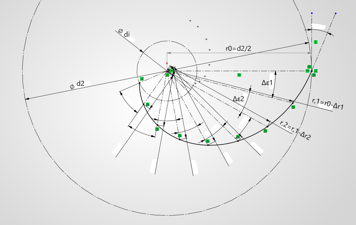
The documented wrap angles are about 209.896° at the hub and 230.502° at the shroud. The reference work gives roughly 130–160° as a usual range for five blades; it is guidance, not a universal limit. A larger outlet metal angle may reduce wrap, but head, width, slip and velocities must then be coordinated again.
Results, messages and next development steps
The screenshots document H₀/H ≈ 1.366, δ₂′ ≈ 13.8° and differing inlet-edge directions. The 1.5-pitch threshold is an internal experimental rule, not the literature wrap-angle range. Messages may be missing or inappropriate; absence of a message is not design approval.
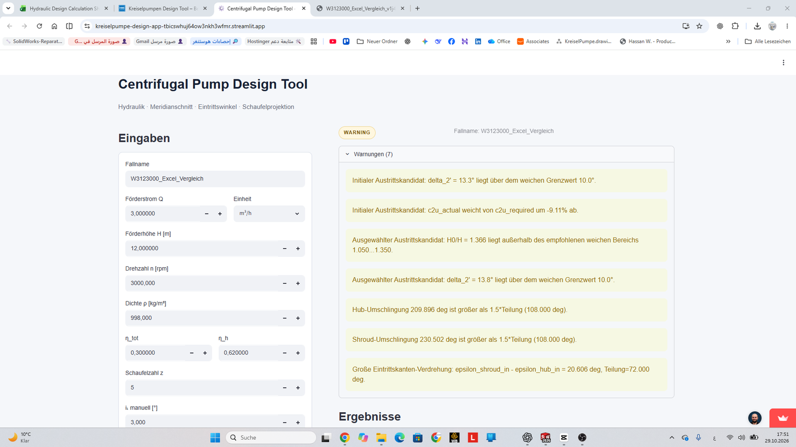
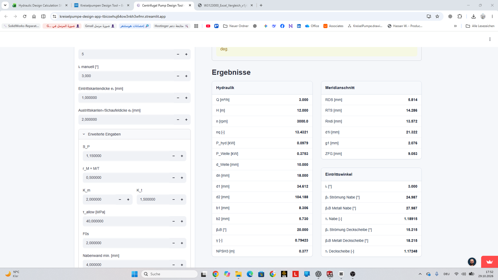
Further development includes checking assumptions and reports, CFD investigation and improvement, and a manufactured, tested prototype. Numerical convergence alone does not prove an optimal design. Casing, bearings, seals, strength and manufacture remain separate design tasks. Feedback should include the case name, complete inputs and report or CSV files.
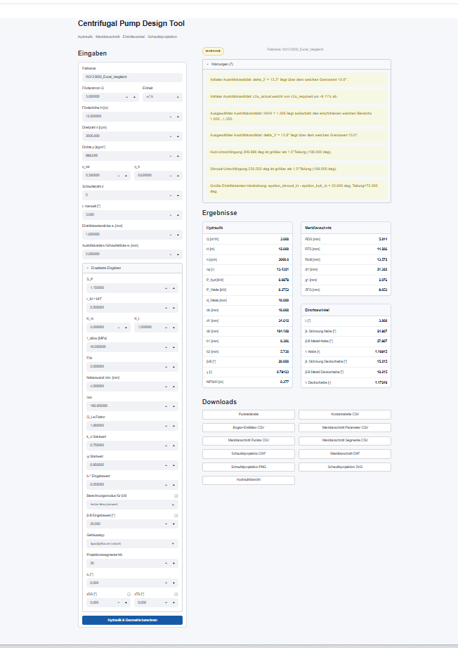
References and technical documentation
The reference is Johann Friedrich Gülich, Centrifugal Pumps, second English edition, Springer, 2010, ISBN 978-3-642-12823-3. Page numbers refer to printed pagination. Example decisions and supplementary Excel models are distinguished from the book relationships.
- Basic equations and power: p. 46, eqs. 2.3–2.4; p. 74, eqs. 3.3–3.5; p. 133, table 3.3.
- Specific speed and suction: p. 82, eq. 3.11; p. 271, eq. 6.7; pp. 273–274; pp. 288–290, eqs. 6.15–6.16 and fig. 6.21.
- Loss types and efficiency: pp. 83–85, 108–109 and 135; hydraulic-efficiency approximation on p. 117, eq. 3.28a. Initial assumptions need assessment through a power and loss balance.
- Inlet, outlet and slip: pp. 131–132, tables 3.1–3.2; definition of d₁m on p. XXIII. Example-specific corrections are explained in the PDF.
- Relative outlet width and meridional section: pp. 345–352, eqs. 7.1–7.2, figs. 7.2 and 7.4; table 7.1 on p. 348.
- Blade design and Kaplan construction: pp. 352–359, eqs. 7.3–7.9 and fig. 7.7. Linear angle distribution and element evaluation are choices for this example.
- Project data: Hydraulic Design Calculation Sheet_W3123000.xlsx, reviewed state of 28 October 2026; Calculations, row 5, and ShaftDiameter. Application screenshots and project drawings: 29 October 2026. No new program run for the comparison table.
Detailed documentation with calculation appendix
German · PDF · 19 pages · 29 October 2026. Includes the complete technical manuscript, assumptions, comparison tables and 22 source notes.
Related resources: Centrifugal pump design project · Calculate specific speed · Estimate installation NPSHA
Limitations and user responsibility
Results are solely for preliminary engineering sizing, plausibility checks and further design, CAD and CFD work. They are not an approved industrial design, a safety assessment or a binding design release.
Use of calculated values, geometry, DXF files, CSV tables and reports is at the user's own responsibility. Before practical or industrial use, qualified specialists must check and validate the results and adapt them to applicable standards, operating conditions, materials, manufacturing processes and safety requirements.
To the extent permitted by law, no liability is accepted for damage, malfunction or defective designs arising from unchecked, improper or out-of-scope use of tool results.
Feedback on the beta version
The tool is deliberately in an early beta phase. This public test version aims to gather practical feedback from engineers, students, lecturers and users in pump engineering and turbomachinery.
Feedback is especially useful on the plausibility of hydraulic values, clarity of inputs and outputs, meridional section display, top-view blade projection and DXF use in CAD systems such as SolidWorks. Reports of possible errors, unclear labels or non-converging designs are also welcome.
Feedback will help progressively improve the methodology, user guidance, documentation and practical usability. The application is an evolving engineering tool for preliminary radial impeller design, rather than a finished product.